Orbital Traffic — Live Sky

Every tracked satellite where it is right now, on a Blue Marble globe, at its true sub-satellite point and its true altitude — rewritten once a second. Hue says which orbital regime an object is in; brightness says whether the Sun is currently shining on it. Nothing here is a simulation: the element sets are the ones the US Space Surveillance Network published this morning, propagated with the standard SGP4 model.

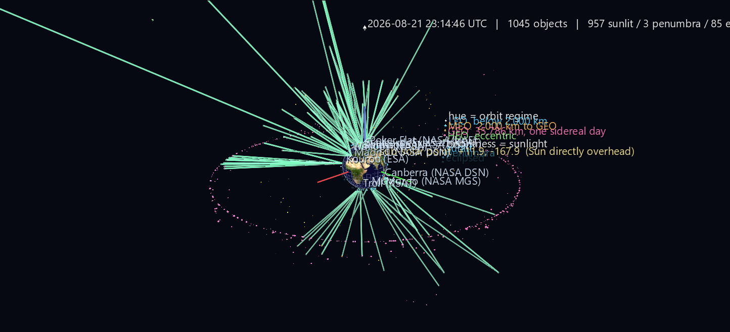
Try it: download this example below (or the full examples set), then open Orbital_Traffic_Example/Live_Sky/live_sky_gv_node.csv — or drag its folder onto the window. Press T for the full label set; Alt+click any satellite to open its CelesTrak catalogue record.

Live_Sky (1 MB)

What you're looking at

Element	Meaning
Globe	World Grid (type 6) in globe form, NASA Blue Marble texture
Small glyphs above it	One per catalogued object, at its real lon/lat/altitude
Glyph hue	Orbit regime — cyan LEO, amber MEO, rose GEO, green eccentric
Glyph brightness	Sunlight: full = lit, half = penumbra, quarter = eclipsed
Glyph shape	Octahedron = payload, cylinder = rocket body, tetrahedron = debris
Glyph size	Radar cross section from the SATCAT, log-compressed
Amber ring on the surface	The day/night terminator — a real great circle, 90° from the Sun
Yellow sphere	The sub-solar point: where the Sun is directly overhead
White pins	Ten real ground stations, on their true coordinates
Green edges	Station → satellite, for the ten highest passes at that station
Caption overhead	UTC clock, object and illumination tallies, element age

1,528 nodes in all: 1,045 objects, 10 stations, the terminator ring, and a fixed pool of 280 link nodes.

The scale is honest, and that is the point

A World Grid globe places children on a sphere of radius 180/π ≈ 57.3 world units, so one world unit is 111.32 km — one degree of latitude. The scene uses that scale straight, with no compression:

Orbit	Altitude	Height above the globe
ISS	419 km	3.8 units — 0.07 Earth radii
Starlink shell	550 km	4.9 units
GPS / Galileo	20,200 km	181 units — 3.2 R
GEO belt	35,786 km	321.5 units — 5.6 R

So the default view is about eleven Earth-diameters across, and Earth is a small ball at the centre of a very large, very empty volume with three distinct inhabited shells in it: a fuzzy layer clinging to the surface, two GNSS shells halfway out, and a razor-thin rose ring at the edge. Rebuild with --max-alt-km 2000 for the LEO close-up.

What to look for

• The ISS is in the dark for 38.7% of its orbit. 36 of every 93 minutes — and that fraction is not fixed. It tracks the beta angle between the Sun and the orbit plane over a roughly 60-day cycle, and near the top of that cycle the station runs for days without a sunset at all.
• A GEO satellite is normally never eclipsed — the belt sits about 12° off the shadow axis in late August, and the umbra only subtends 8.4° there. GEO eclipse season is roughly three weeks either side of each equinox.
• Except for the ones that are. On 21 August 2026 six of 568 GEO objects sat in shadow, all of them within 7.5° of the anti-solar longitude and at latitudes between −3.6° and −10.4°. They are inclined GEO satellites — old birds that have given up north–south stationkeeping and now swing above and below the equator each day, into a shadow their well-stationkept neighbours a few degrees away miss entirely. Two satellites side by side in the same belt, one lit and one dark, for a reason you can see.
• Why polar stations exist. Averaged over 24 hours, LEO objects above 5° elevation: McMurdo (−77.8°) sees 25.1, Svalbard (+78.2°) 24.6, Kiruna 18.8, Madrid 9.7, Kourou (+5.3°) 7.6. A clean monotonic slide with latitude and a 3.3× advantage for the polar sites — most LEO satellites are in near-polar orbits, so their ground tracks converge at high latitude. Svalbard's whole commercial existence is in that column, and running the scene live for a minute shows it happening.
• Most of what a station can see is not worth tracking. Across the ten stations there are 2,065 station–satellite pairs above 5° elevation at once. Restrict the scene to LEO and the same tally drops to 145. A geostationary satellite is visible from about 42% of the planet at once; a 550 km LEO satellite from about 3%.

Going live

python build_live_sky.py --watch 1

Open the scene and turn on File > Watch and Reload (Ctrl+R). The viewer polls the file's mtime once a second and hot-reloads in place, preserving camera, selection and playback. A full frame — propagate 1,045 objects, classify illumination, compute ten stations' worth of look angles, and write 1,528 nodes — takes 31 ms, so the generator is nowhere near the bottleneck. Writes are atomic, so a reload never sees a torn CSV.

Node ids never move, which matters more than it sounds. Every id comes from a fixed layout computed once from the configuration, never from the moment being rendered; objects that fail to propagate or that an altitude filter excludes are written as hidden rows rather than dropped, and the station-link pool is a fixed block whose unused slots are hidden self-links. The set of visible edges churns completely every second while the file's shape never changes — which is what lets you keep a satellite selected and watch its properties update live.

CelesTrak's rate limit

CelesTrak refreshes GP data every 2 hours and temporarily firewalls IPs that poll faster. A too-soon repeat request does not return an error status — it returns HTTP 200 with a plain-text "GP data has not updated since your last successful download" body, which a fetcher that trusts the status code parses as an empty CSV. The example's fetcher sniffs for the OBJECT_NAME header, falls back to its on-disk cache, and never re-requests inside the 2-hour window. --watch only ever re-propagates; it does not re-fetch.

The rest of the set

• One Orbit — the same sky, one full 93-minute revolution precomputed into Channels and replayable in twenty seconds.
• Orbital Shells — the orbital planes themselves, in the inertial frame, turning by themselves.

The example ships four verification suites totalling 54 checks — the physics against independent implementations and published astronomy, and the picture against the real GlyphViz transform engine (globe children land at their written lon/lat/altitude to 2.3 × 10⁻¹³ world units; rendered altitude matches the label to 502 m over 1,045 satellites).

Data and attribution

Orbital data and satellite catalogue courtesy of CelesTrak (Dr. T. S. Kelso, celestrak.org), derived from US Space Surveillance Network observations. Globe texture: NASA Blue Marble. Rebuilding needs the sgp4 package (a 148 KB pure wheel, no build step); the scene as shipped is pure CSV and needs nothing.

SGP4 is good to roughly a kilometre at epoch, degrading 1–3 km/day for LEO. That is right for a visualization and nowhere near good enough for conjunction assessment — don't fly anything using this.