The Century Swarm

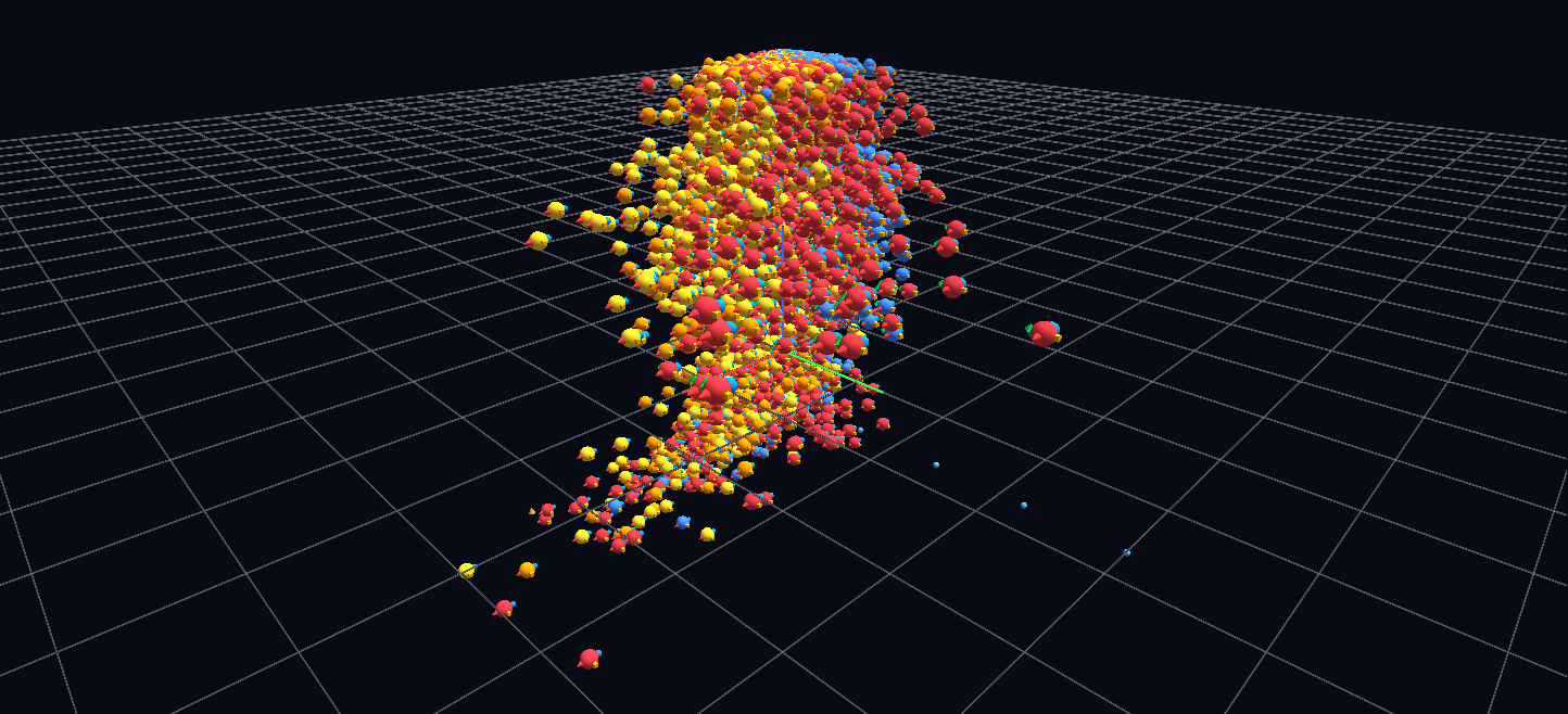
All 29,140 player-seasons of 25+ games from 1921–2012 as hyperglyphs placed in scoring phase space — goals per game × assists per game × year — sized by points per game and colored by position, with stat satellites on each: about 140,000 nodes.

Try it: download this example below (or the full examples set), then open Century_Swarm_Example/century_swarm_gv_node.csv — or just drag its folder onto the GlyphViz window.

Download this example (3 MB)

What it is

Every player-season of 25 or more games in professional hockey from 1921–22 to 2011–12 is one glyph, 29,140 of them, hung in a three-dimensional space that is a scatter plot of how players actually scored. The position of a glyph is the data: nothing is arranged for looks. The result is a single cloud whose shape tells the story of a century of the game.

With its satellites the scene holds about 140,000 nodes, which makes it one of the larger scenes in the gallery. It loads from a single file with no animation, and it is meant to be flown through.

How to read it

The three axes are the three numbers that define a scoring season:

Axis	Meaning
X	goals per game
Y	assists per game
Z	the year, from 1921–22 at one end to 2011–12 at the other

Each season is a sphere, sized by points per game and coloured by position: red for centres, orange and gold for wingers, blue for defensemen and green for goalies. Around each sphere sit small satellites for its goals, assists, penalty minutes and plus/minus, the last signed.

Now look at the cloud rather than at any one glyph:

• A dense mass of ordinary seasons hugs the low corner. Most players, in most years, scored little. The crowd is the baseline.
• The whole cloud breathes with the era. It spreads outward through the 1980s, when scoring soared, and contracts again into the lower-scoring "dead puck" years.
• Defensemen form a blue wall along the low-goals plane. Bobby Orr's seasons are the exception: they escape deep into forward territory.
• The great seasons are detached. The most extraordinary seasons physically separate from the swarm. Remoteness from the crowd is the ranking, so you can find the all-time greats by flying outward until you reach something alone.

Click any glyph to read that player-season's full line. A handful of guide labels (the decades along the year axis) mark the way, because in unlabelled space it is easy to lose your bearings.

Things to try

• Open it with tag labels off, which is how the scene is meant to be read. At this density a label for every glyph would bury the scene, so each glyph shows its line only when selected.
• Fly the year axis. Start at the first season and travel along Z: the cloud swells and thins as eras pass.
• Look for the outliers at the far edges. Each one is a season that has no neighbours.

How it is built

The hierarchy is deliberately flat: one root, about 29,000 season spheres (and a few guide nodes) and about 111,000 satellites, two levels deep. Position is carried by the glyphs' own coordinates in space instead of by topology scaffolding, which is the right design for a scatter plot. The cloud fits in a bounded volume of about ±26 units, so nothing clips when you fly around it.

A few details are worth borrowing if you build a big scene yourself. Rendered sizes are kept above the 0.2 floor even through the multiplication of parent and satellite scales (a parent of at least 0.6 times a satellite of at least 0.34 keeps every product above 0.204), so no glyph vanishes. And at this density, inline labels shown only for a selection are the only labelling strategy that works.

The generator, build_swarm.py, ships with the scene and reads the hockey history CSVs named by its HOCKEY_DATA setting.